|
|
Why graphs
- relations of entities
- Similar data points
- arbitrary sizes, no spatial index,
- no reference order
- representation learning
- Map nodes to d-dimensional embeddings-> similar nodes in the network are embedded close together
Applications of Graph ML
- different tasks:
- Node classification
- Link prediction: knowledge graph completion
- Graph classification: molecule property prediction
- Clustering
- Graph generation
- Graph evolution: physical simulation
- Examples:
- node-level: Protein folding
- Recommender system: recommend related pins to users by edge level classification
- subgraph-level: traffic prediction: nodes: road segments, edges: connectivity between nodes-> predict time arrival etc
- graph-level: drug discovery: nodes: atoms, edges: chemical bonds. graph generation, generate new molecules in a targeted way.
- physicalsimulation: nodes: particles, edges interactions between particles-> predict how a graph will evolve over.
Choice of Graph representation
- Node degree (ubdirected): the number of edges adjacent to node i
- in-degree, out-degree(directed)
- Bipartite graph: two disjoint sets U and V. e. author to papers. two different type of nodes
- Adjacency matrix. For a directed graph, adjacency matrix is not symmetric
- Adjacency sparse for most real-word networks.
- represent as a list of edges.
- represent as an adjacency list
- node and edge attributes: weight, ranking, type, sign, etc.
- weighted and unweighted adjacency matrix.
- self-loop node, multigraph->adjacency matrix different.
- connected graph: any two nodes canbe joined by a graph.
- A graph with mutiple components: adjacency matrix can be written in a block way.
- Strongly connected directed graph: has a directed path to every other node. weakly connected directed: is connected if disregard the edge direction
- strongly connected directed components: in the component, it is strongly connected.
Traditional methods: Node
- hand-designed features
Node-level
- node degree
- node centrality:
- A node is important if surrounded by important neighboring nodes $u\in N(v)$ $$c_v = \frac{1}{\lambda}\sum_{u\in N(v)}c_u \rightarrow \lambda \mathbb{c}=\mathbb{Ac}$$ Where &A& is adjacency matrix.
- Clossness centrality:
- clustering coefficient: count triangles that a node touches
- graphlets:
- graph degree vector: counts the occurence of the graphlets
Link-level
- the key is design of the feature of pair nodes.
- Links missing prediction
- links overtime prediction
- compute score c(x,y)-> sort score-> keep top k
- representation:
- shortest path between two nodes.
- common neighbors between two nodes
- jaccard’s coefficient
- Adamic-adar index
- Global neighborhood overlap:
- computing number of paths between two nodes: can be obtained by computing power of adjacency matrix
- power: $P^{(K)} = A^K$-> means # paths of length K between $u$ and $v$.
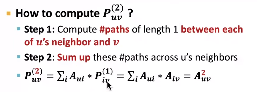
- katz index:$S_{v_1 v_2} = \sum_{l=1}^{\inf}\beta^lA_{v_1 v_2}^l$
- katz index matrix: $S=\sum_{i=1}^{\inf}\beta^i A^i= (I-\beta A)^{-1}-I$
graph-level
- features to characterize the structure of an entire graph
- Kernel methods: $K(a,b) = \phi(a)^T\phi(b)$. kernel matrix K has to be semi-definite and can be orthogonally decomposed.
- goal: design graph feature vector $\phi(G)$
- Key idea: bag of words for a graph.
- bag of degrees nodes
- graphlet kernel: # different graphlets in a graph.
- graphlets list(g1,g2,g3,…) (not need to be connected different from nodel-level graphlets which has to be connected) -limitations: counting graphlets is expensive
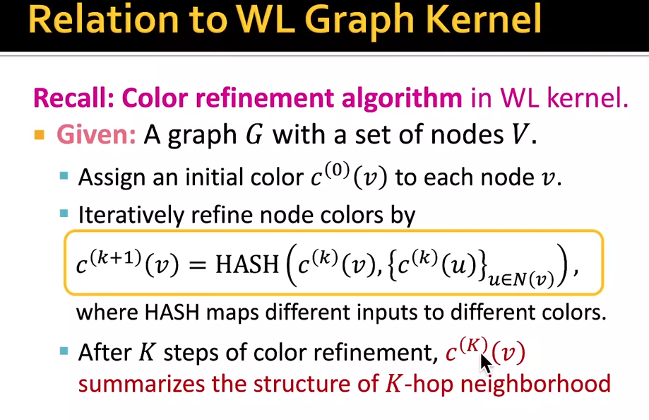
- weisfeiler-Lehman kernel
- goal: design an efficient graph feature desciptor
- idea: use neighborhood structure to iteratively enrich node vocabulary.-> color refinement
- $c^{k+1}(v) = HASH({c^{k}(v), {c^k(u)}}_{u\in N(v)})$. HASH maps input to colors. K steps summarize the structure of k-hop neighborhood
Node embedding
eg. 2d embedding of nodes of the Zachary’s Karate Club network from “Deepwalk:Online learning of social representations”
- key idea: define a node similarity function
- $P(v|z_u)$ the probability of visiting node v on random walk starting from the node u.
- Softmax function/Sigmoid
- Random walk; $z_u^Tz_v$ probability u and v cooccur at a random walk
- unsupervised feature learning: maximize log-likelihood: $\max_f\sum_{u\in V}logP(N(u)|Z_u)$
- Given a node U, we want to learn feature representations that are predictive of the nodes in its random walk neighborhood $N_R(u)$, wehere R is ramdom walk strategy
- Intuition: optimize embeddings to maximize the likelihood of random walk co-occurrences
- Negative sampling: $P(v|z_u) = softmax(z_u^Tz_v)\rightarrow log(\frac{exp(z_u^Tz_v)}{\sum_{n\in V}exp(z_u^Tz_n)})\rightarrow log(\sigma(z_u^Tz_v))-\sum_{i=1}^k\log(\sigma(z_u^Tz_{n_i})), n_i~P_V, \sigma Sigmoid$
- NCE approximation
- How to select strategy
- Node2vec:
- local and global: BFS and DFS
- biased fixed-length random walk:
- 2-nd order random walks: return/ BFS/DFS
- two parameters: p and q
- parallelizable
- Node2vec:
Embed entire graph
- simple idea: just sum up the node embeddings in the graph-> classification
- Virtual node to represent the (sub)graph
- Anonymous walk embeddings
- represent the graph as a probability distribution over these walks
- Learn walk embeddings
PageRank, random walk and embeddings
- $r = Mr$ for directed graph.
- eigen vector centrality: $\lambda c = Ac$ for undirected graph.
Random walk with restarts and personalized pagerank
- Personalized pagerank: ranks proximity of nodes to the teleport nodes S.
- idea every node has importance; importance gets evenly split among all edges and pushed to the neighbors.
Matrix factorization
above all random walk based methods
Graph neural network
Message passing and node classification
- Correlation: nearby nodes same class
- Homophily: the tendency of individuals to associate and bond with similar others. Influence: social connections can influence the individual charactersictis of a person
Relational classification and Iterative classification
- Relational: class probability of node v is a weighted average of class probability of its neighbors.
- Iterative: use attributes and labels of neighbor nodes.
Collective classification
- A dynamic programming approach answering probability queries in a graph
- iterative way: neighbor nodes talk to each other.
- I believe you belong to class 1 with likelihood.
Graph neural networks
- Encoder: $z(v) = ENC(v)$, decoder: similarity function.
- can also embed subgraphs, graphs
- modern depplearning tool box is designed for simple sequences and grids.
- networks: arbitrary size, complex topological structure, no fixed ordering or reference point, dynamic
Deep learning for graphs
- A naive appproach
- join adjacency matrix and features
- Challenges: no ordering nodes, how to use convolutiuon
- Solution: $\sum W_i h_i$. Node’s neighborhood defines a computation graph.
- step 1, define computation graph
- step 2, propagat einformation.
- Aggregate neighbors: nodes aggregate information from their neighbors using neural network.
- Every node define a computation graph based on its neighborhood.
- Model can be of arbitrary depth. Only do for limited steps. layer-k embeddings get k-hop information.
- Permutation invariant
- How to train the model: feed embedding into any loss function and run SGD to train the parameters.
- Unsupervised settingL use the graph structure as the supervision. $L = \sum_{z_u,z_v}CE(y_{u,v},DEC(z_u, z_v))$
A general perspective on GNN
- GNN layer = Message + Aggregation
A single layer of GNN
- GraphSAGE: $h_v^{(l)} = \sigma(w^{(l)}\cdot CONCAT(h_v^{(l-1)}, AGG({h_u^{(l-1)},\forall u \in N(v)})))$
- Graph attention networks: $h_v^{(l)} = \sigma(\sum_{u\in N(v)}\alpha_{vu}W^{(l)}h_u^{(l-1)})$, where $a_{vu}$ is attention weight. in graphSAGE, it is $\frac{1}{|N(v)|}$
- multi-head attention: $a_{vu}^1, a_{vu}^2,a_{vu}^3$
Stacking layers of a GNN
- GNN suffers from over-smoothing problem: all the node embeddings coverge to the same value.
- Why it happens: the receptive of the GNN is too big, so all the node receive the same information, so the final output tend to be the same.
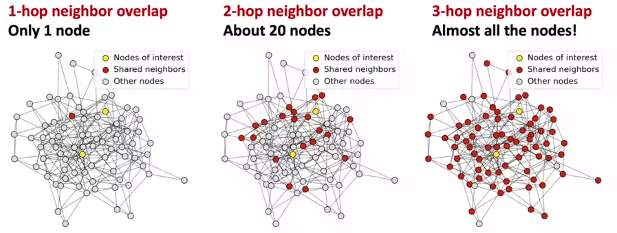
- Explanation: two nodes have highly overlapped receptive fields, their embeddings are highly similar.
- Overcome: be cautious when adding GNN layers.
- Increase the expressive power within each GNN layer: linear aggregation to non-linear/ deep neural network.
- Add layers do not pass messages.
- Add skip connection in GNNs
Graph augmentation
- Idea: Raw input graph $\neq$ computational graph
- graph feature augmentation: input graph lacks features-> feature computation
- graph structure augmentation: too sparse, too dense, too large->add virtual nodes/edges
- it is unlikely the input graph to be the optimal computational graph.->sample subgraphs
- Feature augmentation:
- input graph doesn’t have node fatures:
- assign constant values to nodes
- assign IDs to nodes and onr-hot encoding
- node cannot differentiate the circle and infinitely long series
- Use cycle count as node features:[0,0,0,1,0,0] and [0,0,0,0,1,0]
- input graph doesn’t have node fatures:
- Structure augmentation
- Add virtual edges:
- connect 2-hop neighbors via virtual edges
- intuition: adjacency matrix: $A+A^2$
- Add virtual nodes:
- in a sparse graph the fdistance too large
- adding virtual nodes, distance will be two
- Node neighborhood sampling
- sample a node’s neighborhood for messgae passing
- Add virtual edges:
Train a GNN
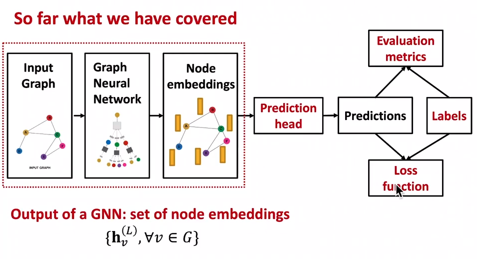
- prediction head:
- node-level tasks
- edge-level tasks
- graph-level tasks
- options for edge:
- concatenation of $h_u, h_v$ + Linear prediction
- dot product: $\hat{y}_{uv} = h_u\cdot h_v$
- graph-level prediction
- make prediction using all node embeddings
- options
- global mean pooling
- global max pooling
- global sum pooling
- issues
- lose information
- hierarchical pooling: aggregate partially and then aggregate aggregations
- supervised vs unsupervised
- e.g. link prediction
- Unsupervised -> self-supervised
Setting up graph training
-
each data point is a node, test data influence prediction on training data
-
options:
- transductive settings: the graph structure can be observed over all stages
- inductive setting: different graphs for different stages
-
link prediction: self-supervised
- two kinds of edges: message passing and predictive edges
- transductive or inductive setting
How expressive are graph neural networks
- Key idea: generate node embedding based on local network neighborhoods
- Intuition: Nodes aggregate information from neighbors using NN
how powerful are GNNs
- proposed: GCN, GAT, graphsage, design space
- GCN: Meanpooling
- GraphSAGE: max pooling
- How well can a GNN distinguish different graph structures
- can GNN node embeddings distinguish different node’s local neighborhood structures? if so, when? if not when will a GNN fail?
- How a GNN captures local neighborhood structure?-> computational graph.
- computational structure = rooted subtree structure
- Injective function:
- function: injective if it maps different elements into different outputs.
- it retains all information of the input
- Most expressuve GNN should map subtrees to the node embeddings injectively.
- If each step of GNN’s aggregation can fully retain the neighboring information the generated node embeddings can distinguish different rooted subtrees
- In another words, most expressive GNN would use an injective neighbor aggregation function at each step.
Design the most expressive GNN
- key idea: expressive power of GNNs can be characterized by that of neighbor aggregation functions they use.
- ObeservationL neighbor aggregation can be abstracted as a function over a multi-set
- GCN: $Mean({x_u}{u\in N(v)})$, GraphSAGE: $Max({x_u}{u\in N(v)})$
- GCN & GraphSAGE cannot distinguish different multi-sets with the same color proportion.
- Any injective multi-set function can be expressed as :$\phi(\sum_{x\in S}f(x))$, where $\phi, f$ refer to non-linear function
- Graph Isomorphism Network
relation to WL kernel
Heterogeneous graphs
- relational GCNs, Knowledge graph, embeddings for KG Completion
- $G = (V,E,R,T)$, nodes, edges, node type, relation type
- Relational GCn
- multiple edge types
- recap GCN:
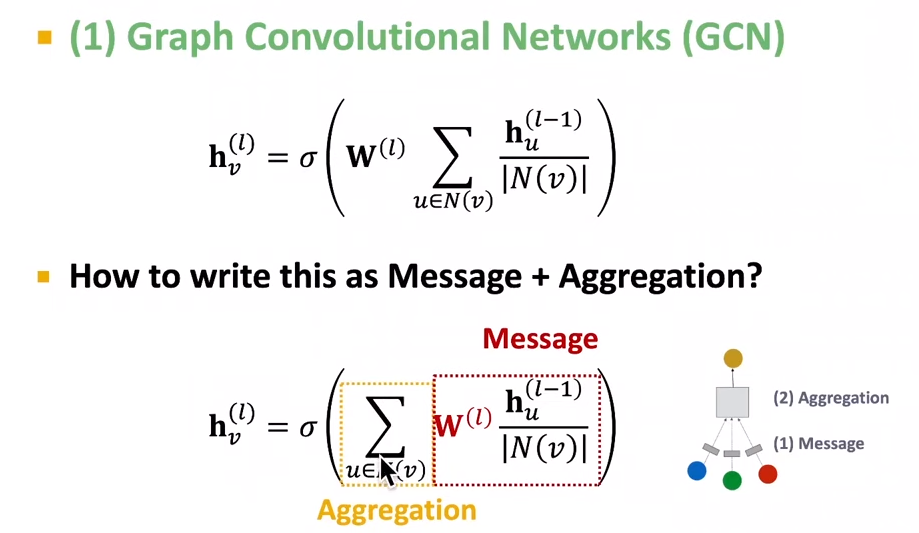
- what if the GCN has multiple relation types
- Use different network weights for different relation types:$h_v^{(l+1)} = \sigma(\sum_{r\in R}\sum_{u \in N_v^r}\frac{1}{C_{v,r}}W_r^{(l)}h_u^{(l)}+W_0^{(l)}h_v^{(l)})$
- Share weights across relations
- represent the matrix of each relation as a linear combination of basis transformations
- $W_r = \sub_b a_{rb}V_b$, where $V_b$ is share across all relations, so each relation only needs to learn $a_{rb}$
- link prediction:
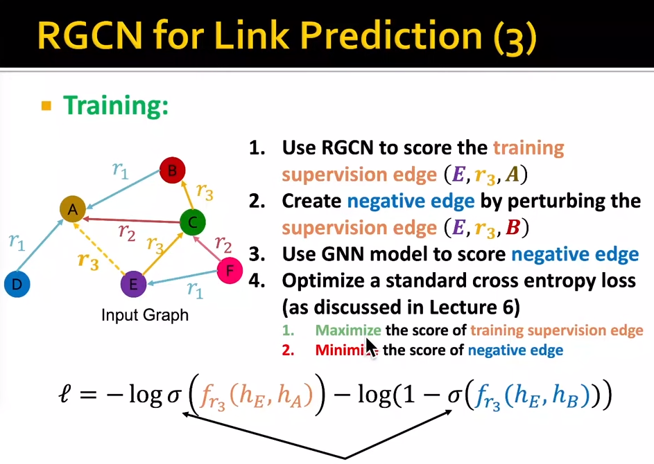
Knowledge graph completion
- KG in graph: entities, types, relationships.
- KG task: predict the missing tails.
- shallow encoding: the encoder is just an embedding lookup
- KG representation: (head relation, tail)=(h,r,t)
- given the (h,r,t), the embedding (h,r) should be close to t.
- scoring function: $f_r(h,t) = -||h+r-t||$
- relations in a heterougeneous KG have different properties.
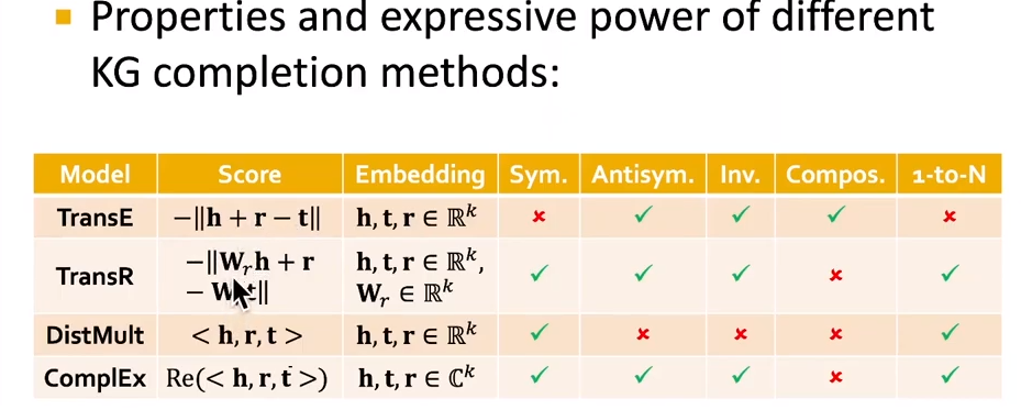
- relation patterns:
- symmetric, antisymmetric, inverse, composition, 1-to-N
- antisymmetric:
- TansE cannot model symmetric or antisymmetric, 1-to-N
- TransR:
- $h^\prime = M_r h, t^\prime = M_r t$
- scoring function: $f_r(h,t) = -||h^\prime+r-t^\prime||$
- DisMult: cannot model antisymmetric, inverse, compositional. scoring function (hrt)
- ComplEx
Reasoning in KG
- Goal: How to perform multi-hop reasoning over KGs
- one-hop, path, conjunctive
- KG incompleteness is not able to identify all anser entities.
Answering in KGs
- TransE: $a = v_a + r_1 + r_2 + \cdots$, TransR, DistMult, ComplEx cannot handle the path queries
KGs and Box embeddings:
- entity embeddings: entites are seen as a zero-volume boxes
- relation: each relation takes a box and produces a new box:
Generative models for graphs
- motivation for graph generation: we want to generate realistic graph
- understand formulation of graphs
- predictions graph
- use same process to general novel graph instances
- Road map
- properties of real-world graphs
- traditional fraph generative models
- deep graph generative models
- propertites:
- degree distribution: probability a randomly chosen node has degree k
- clustering coefficient: how connected are i’s neighbors to each other
- connectivity: size of the largest connected component
- Path length: 90% within 8 hops-> small world model
Erdos-Renyi Random Graphs
- $G_{np}$ undirected graph on n nodes where each edge iid with probability -.
- propertities:
- Degree distribution: binomial distribution
- clustering coefficient
- path length
Deep grah generation
- generate graph are similar to a given set of graphs
- goal-direted graph generation
- given $p_{data}(G)$ learn the distribution $p_{model}(G)$
- sample $p_{model}(G)$
- the most common approach: sample $z_i$ and transform to graph $x$ with $f(z_i)$
- auto-regressive models: $p_{model}(x;\theta)$ is used for both density estimation and sampling. (VAE and GAN have 2 or more models, each playing one of the rules)
- idea: chain rule. $p_{model}(x;\theta) = \prod_{t=1}^n p_{model}(x_t|x_1,x_2, \cdots, x_{t-1};\theta)$ where $x_t$ will be the t-th action (add node, add edge)
GraphRNN
-
generating graphs via sequentially adding nodes and edges.
- node-level: add nodes, one at a time
- edge-level: add edges
- each node step is an edge sequences. each time add a new node, decision on edge connection to every former nodes has to be made.
- Summary: a graph + a node ordering = a sequence of sequences.
- transform to a sequence generation problem-> RNN
- has a nodel-level RNN adn an edge-level RNN
-
scaling up by Breadth First Search (BFS)
-
Compare sets of training graph statistics and generated graph statistics
- how to compare two graph statistics: Earth mover distance
- how to compare sets of graph statistics: Maximum Mean Discrepancy
-
Earth mover distance: measure the minimum effort that move earth from one pile to the other.
-
Maximum Mean Discrepancy:
Application of deep graph generation
- molecule generation
- GCPN: use reinforcement learning to decide whether take action to link two nodes.
Position-aware GNN
- structure-aware task
- position-aware task: use anchor nodes to locate nodes in the graph
- more anchors can better characterize node position in different regions of the graph.
Identity-aware GNN
- assign a color to the node we want to embed
- heterogenous message passing: another GNN applies different message to nodes with different colorings.
scaling up GNNS
- when nodes too many, hard to train
- GraphSAGE neighbor sampling randomly sample M nodes, get k-hop neighborhood of each node, tehn construct computational graph to train.
- sampling at most H neighbors at each hop to reduce computaion complexity.
- cluster GCN
- sample a small subgraph of the large graph and perform layer-wise node embeddings
- simplifying GCN